We’ll start by creating a data dictionary so that we can refer to it later in our cleaning and data analysis. We do this by creating a data frame or ‘tibble’ because this is a convenient format for manipulating the information.
Now, we write a short description of each variable in the data file.
Code
acuity_data_dict <- acuity_data_dict |> dplyr::mutate(col_desc =c("Last name of 1st author","Full APA format citation","Paper publication year","Source in paper","Reported age range in mos","Age in mos as conformed by ROG","Participants tested monocularly or binocularly","Typical or atypically developing","Number of participants in group","Testing distance in cm","Starting card in cyc/deg","Mean (group) acuity in cyc/deg","Estimated lower limit of acuity in cyc/deg","Teller Acuity Card closest equivalent to this lower limit","Estimated upper limit of acuity in cyc/deg","Country where data were collected","TAC-I or TAC-II"))acuity_data_dict |> knitr::kable(format ='html') |> kableExtra::kable_classic()
col_name
col_desc
author_first
Last name of 1st author
citation
Full APA format citation
pub_year
Paper publication year
fig_table
Source in paper
age_mos
Reported age range in mos
age_grp_rog
Age in mos as conformed by ROG
binoc_monoc
Participants tested monocularly or binocularly
typ
Typical or atypically developing
n_participants
Number of participants in group
distance_cm
Testing distance in cm
start_card_cyc_deg
Starting card in cyc/deg
mean_acuity_cyc_deg
Mean (group) acuity in cyc/deg
lower_limit_cyc_deg
Estimated lower limit of acuity in cyc/deg
closest_card_cyc_deg
Teller Acuity Card closest equivalent to this lower limit
upper_limit_cyc_deg
Estimated upper limit of acuity in cyc/deg
country
Country where data were collected
card_type
TAC-I or TAC-II
Data visualization
Important
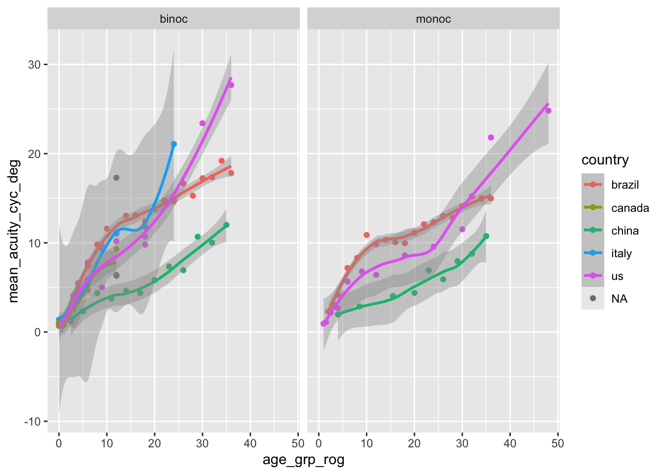
Rick Gilmore decided to take the mean of the age range reported in the (Xiang et al., 2021) data and create a new variable strictly for visualization purposes, age_grp_rog.
We are still in the early phases of the project (as of 2025-04-22 16:35:40.396537), but it is good to start sketching the the data visualizations we will eventually want to see.
Warning in simpleLoess(y, x, w, span, degree = degree, parametric = parametric,
: reciprocal condition number 3.2363e-17
Warning in predLoess(object$y, object$x, newx = if (is.null(newdata)) object$x
else if (is.data.frame(newdata))
as.matrix(model.frame(delete.response(terms(object)), : pseudoinverse used at 3
Warning in predLoess(object$y, object$x, newx = if (is.null(newdata)) object$x
else if (is.data.frame(newdata))
as.matrix(model.frame(delete.response(terms(object)), : neighborhood radius 3
Warning in predLoess(object$y, object$x, newx = if (is.null(newdata)) object$x
else if (is.data.frame(newdata))
as.matrix(model.frame(delete.response(terms(object)), : reciprocal condition
number 3.2363e-17
Figure 4.1: Developmental time course of mean acuity as assessed by Teller Acuity Cards
Call:
lm(formula = mean_acuity_cyc_deg ~ age_grp_rog, data = binoc)

Residuals:
    Min      1Q  Median      3Q     Max
-7.0682 -1.3940 -0.5624  1.3503  9.9061

Coefficients:
            Estimate Std. Error t value Pr(>|t|)
(Intercept)  1.73305    0.46733   3.708 0.000337 ***
age_grp_rog  0.47174    0.02844  16.587  < 2e-16 ***
---
Signif. codes:  0 '***' 0.001 '**' 0.01 '*' 0.05 '.' 0.1 ' ' 1

Residual standard error: 3.131 on 104 degrees of freedom
Multiple R-squared:  0.7257,    Adjusted R-squared:  0.723
F-statistic: 275.1 on 1 and 104 DF,  p-value: < 2.2e-16
Code
summary(lm_m)
Call:
lm(formula = mean_acuity_cyc_deg ~ age_grp_rog, data = monoc)

Residuals:
    Min      1Q  Median      3Q     Max
-5.2832 -1.5766 -0.1751  1.7396  7.1450

Coefficients:
            Estimate Std. Error t value Pr(>|t|)
(Intercept)  2.16669    0.74315   2.916  0.00538 **
age_grp_rog  0.34717    0.03356  10.346 8.22e-14 ***
---
Signif. codes:  0 '***' 0.001 '**' 0.01 '*' 0.05 '.' 0.1 ' ' 1

Residual standard error: 2.755 on 48 degrees of freedom
Multiple R-squared:  0.6904,    Adjusted R-squared:  0.684
F-statistic:   107 on 1 and 48 DF,  p-value: 8.215e-14
By-individual data
The Gilmore lab has some archival data that we can potentially use in this project. The following represents Rick Gilmore’s work to gather, clean, and visualize these data.
Gathering
The de-identified archival data are stored in a Google sheet accessed by the lab Google account.
First, we must authenticate to Google to access the relevant file and download it.
Don't know how to automatically pick scale for object of type <difftime>.
Defaulting to continuous.
`geom_smooth()` using formula = 'y ~ x'
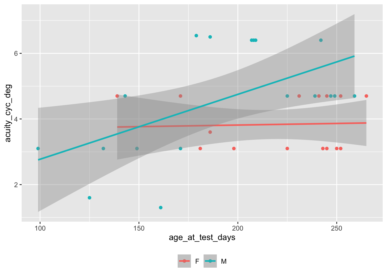
Figure 4.2: Individual participant Teller Acuity Card thresholds from archival Gilmore lab data
Note
Before I stop, I’m going to add the by-participant data file to a .gitignore file, just to be extra careful.
Xiang, Y., Long, E., Liu, Z., Li, X., Lin, Z., Zhu, Y., … Lin, H. (2021). Study to establish visual acuity norms with teller acuity cards II for infants from southern china. Eye, 35(10), 2787–2792. https://doi.org/10.1038/s41433-020-01314-y
Source Code
---title: ""params: data_dir: "data/csv" update_data: TRUE use_sysenv_creds: TRUE google_data_url: "https://docs.google.com/spreadsheets/d/1UFZkbh9oU4JHpYsrkDQcNmDyqD4J-qB74dhyMzIkqKs/edit?usp=sharing" sheet_name: "typical_group" data_fn: "typical_group.csv"---## OverviewThis page describes the process of data gathering, cleaning, and visualization.## GatheringWe use a Google Sheet to store the by-study data:<https://docs.google.com/spreadsheets/d/1UFZkbh9oU4JHpYsrkDQcNmDyqD4J-qB74dhyMzIkqKs/edit#gid=0>::: {.callout-note}**Note**: There is no identifiable data here at the moment, so Google Sheets are a viable option.Later on, we start contacting authors, we will need to restrict access to that information for privacy reasons.:::::: {.callout-important}We need a process for managing who has edit access.:::The [`googledrive`](https://cran.r-project.org/web/packages/googledrive/index.html) package provides a convenient way to access documents stored on Google.### Download from Google as CSV```{r}if (!dir.exists(params$data_dir)) {message("Creating missing ", params$data_dir, ".")dir.create(params$data_dir)}if (params$update_data) {if (params$use_sysenv_creds) { google_creds <-Sys.getenv("GMAIL_SURVEY")if (google_creds !="") {options(gargle_oauth_email = google_creds) googledrive::drive_auth() } else {message("No Google account information stored in `.Renviron`.")message("Add authorized Google account name to `.Renviron` using `usethist::edit_r_environ()`.") } } this_sheet <- googlesheets4::read_sheet(ss = params$google_data_url,sheet = params$sheet_name) out_fn <-file.path(params$data_dir, params$data_fn) readr::write_csv(this_sheet, out_fn)message("Data updated: ", out_fn)} else {message("Using stored data.")}```The data file has been saved as a comma-separated value (CSV) format data file in a special directory called `csv/`.### Open CSVNext we load the data file.```{r, message=FALSE, echo=TRUE}acuity_df <- readr::read_csv(file.path(params$data_dir, "by-paper.csv"), show_col_types = FALSE)```We'll show the column (variable names) since these will be part of our data dictionary.```{r}acuity_cols <-names(acuity_df)acuity_cols```### Create data dictionaryWe'll start by creating a data dictionary so that we can refer to it later in our cleaning and data analysis.We do this by creating a data frame or 'tibble' because this is a convenient format for manipulating the information.```{r}acuity_data_dict <- tibble::tibble(col_name =names(acuity_df))```Now, we write a short description of each variable in the data file.```{r}acuity_data_dict <- acuity_data_dict |> dplyr::mutate(col_desc =c("Last name of 1st author","Full APA format citation","Paper publication year","Source in paper","Reported age range in mos","Age in mos as conformed by ROG","Participants tested monocularly or binocularly","Typical or atypically developing","Number of participants in group","Testing distance in cm","Starting card in cyc/deg","Mean (group) acuity in cyc/deg","Estimated lower limit of acuity in cyc/deg","Teller Acuity Card closest equivalent to this lower limit","Estimated upper limit of acuity in cyc/deg","Country where data were collected","TAC-I or TAC-II"))acuity_data_dict |> knitr::kable(format ='html') |> kableExtra::kable_classic()```## Data visualization::: {.callout-important}Rick Gilmore decided to take the mean of the age range reported in the [@Xiang2021-ry] data and create a new variable *strictly* for visualization purposes, `age_grp_rog`.:::We are still in the early phases of the project (as of `r Sys.time()`), but it is good to start sketching the the data visualizations we will eventually want to see.```{r fig-teller-acuity-across-age, fig.cap="Developmental time course of mean acuity as assessed by Teller Acuity Cards"}library(ggplot2)acuity_df |> ggplot() + aes( x = age_grp_rog, y = mean_acuity_cyc_deg, color = country ) + geom_point() + geom_smooth() + facet_grid(cols = vars(binoc_monoc))```Number of total participants.```{r}#| label: cross-tabsacuity_df |> dplyr::filter(!is.na(n_participants)) |> dplyr::mutate(n_participants_tot =sum(n_participants)) |> dplyr::select(n_participants_tot) |>unique()``````{r}acuity_df |> dplyr::group_by(age_grp_rog) |> dplyr::mutate(min_acuity =min(mean_acuity_cyc_deg),max_acuity =max(mean_acuity_cyc_deg),max_minus_min = max_acuity - min_acuity) |> dplyr::select(age_grp_rog, min_acuity, max_acuity, max_minus_min) |> dplyr::arrange(age_grp_rog) |> kableExtra::kable(format='html') |> kableExtra::kable_classic()``````{r}binoc <- acuity_df |> dplyr::filter(binoc_monoc =="binoc")monoc <- acuity_df |> dplyr::filter(binoc_monoc =="monoc")lm_b <-lm(mean_acuity_cyc_deg ~ age_grp_rog, data = binoc)lm_m <-lm(mean_acuity_cyc_deg ~ age_grp_rog, data = monoc)summary(lm_b)summary(lm_m)```## By-individual dataThe Gilmore lab has some archival data that we can potentially use in this project.The following represents Rick Gilmore's work to gather, clean, and visualize these data.### GatheringThe de-identified archival data are stored in a Google sheet accessed by the lab Google account.First, we must authenticate to Google to access the relevant file and download it.```{r}options(gargle_oauth_email ="psubrainlab@gmail.com")googledrive::drive_auth()```Then we download the relevant file.```{r}googledrive::drive_download("vep-session-log",path =file.path(params$data_dir, "by-participant.csv"),type ="csv",overwrite =TRUE)```Unlike the Google sheet newly created for the by-study data, this one requires a lot of cleaning.```{r}gilmore_archival_df <- readr::read_csv(file.path(params$data_dir, "by-participant.csv"),show_col_types =FALSE)names(gilmore_archival_df)```We'll keep `Date`, `Time`, `Sex`, `DOB`, `Teller Acuity Cards`, `Age at test`.```{r}gilmore_archival_df <- gilmore_archival_df |> dplyr::select(Date, Time, Sex, DOB, `Teller Acuity Cards`, `Age at test`)```Then, let's filter those where we have TAC data.```{r}with(gilmore_archival_df, unique(`Teller Acuity Cards`))``````{r}gilmore_archival_df <- gilmore_archival_df |> dplyr::filter(!is.na(`Teller Acuity Cards`),`Teller Acuity Cards`!="not interested")dim(gilmore_archival_df)```::: {.callout-note}This file illustrates how making data FAIR from the outset can save work.This one is not too terribly hard to parse, but it could have been better planned.:::We'll extract the viewing distance with a regular expression.```{r}gilmore_archival_df <- gilmore_archival_df |> dplyr::mutate(view_dist_cm = stringr::str_extract(`Teller Acuity Cards`, "[0-9]{2}cm")) |> dplyr::mutate(view_dist_cm = stringr::str_remove(view_dist_cm, "cm")) # remove 'cm'gilmore_archival_df$view_dist_cm```Similarly, we'll extract the acuity in cyc/deg using a regular expression.```{r}gilmore_archival_df <- gilmore_archival_df |># add 'cyc' to separate cyc/deg from Snellen acuity dplyr::mutate(acuity_cyc_deg = stringr::str_extract(`Teller Acuity Cards`, "[0-9]{1}[\\./]{1}[0-9]+ cyc")) |> dplyr::mutate(acuity_cyc_deg = stringr::str_remove(acuity_cyc_deg, " cyc")) |> dplyr::mutate(acuity_cyc_deg = stringr::str_replace(acuity_cyc_deg, "/", "."))gilmore_archival_df$acuity_cyc_deg```Now, let's look at the age at test.```{r}gilmore_archival_df$`Age at test````Instead, let's see what it looks like to compute age at test from the dates.```{r}gilmore_archival_df <- gilmore_archival_df |> dplyr::mutate(age_at_test_days = lubridate::mdy(Date) - lubridate::mdy(DOB))gilmore_archival_df$age_at_test_days```That seems reasonable for now.Let's see if we can plot these data.```{r fig-gilmore-lab-archival, fig.cap="Individual participant Teller Acuity Card thresholds from archival Gilmore lab data"}gilmore_archival_df |> dplyr::mutate(acuity_cyc_deg = as.numeric(acuity_cyc_deg)) |> ggplot() + aes(x = age_at_test_days, y = acuity_cyc_deg, color = Sex) + geom_point() + geom_smooth(method = "lm") + #theme_classic() + theme(legend.position = "bottom", legend.title = element_blank()) ```::: {.callout-note}Before I stop, I'm going to add the by-participant data file to a `.gitignore` file, just to be extra careful.:::